a. mean?
b. median?
c. standard deviation?
If you instead multiply the original value of each observation by 2, what are the new values of the
d. mean?
e. median?
f. standard deviation?
2. A study looked at a random sample of 100 companies whose stocks were traded on the New York Stock Exchange (NYSE). The companies were divided into quintiles (the 20 largest companies, the 20 next largest, and so on) and the stock market rates of return over the preceding 20 years were calculated for each quintile. This study found that the quintile with the smallest companies (“small-cap” stocks) had done better than the quintile with the largest companies (“large-cap” stocks). Identify the most important statistical bias in this sample and explain how the study could be redone to get rid of this problem.
3. A September 9, 2009 article in the New York Times argued that one reason many students don’t graduate from college within six years of enrolling is that they choose to “not attend the best college they could have.” For example, many students with a 3.5 high school grade-point average could have gone to the University of Michigan Ann Arbor, which has an 88% graduation rate, but choose instead to go to Eastern Michigan, which has only a 39% graduation rate.
a. What flaws do you see in the implication that these students would have a better chance of graduating if they went to the University of Michigan instead of Eastern Michigan?
b. What kind of data would we need to draw a valid conclusion?
4. Suppose that 10 percent of all investment advisers are experts and 90 percent are guessers. Each expert has a 0.6 probability of making a correct prediction whether the stock market will beat the bond market over the course of a year; a guesser has a 0.5 probability of being correct. Each adviser’s chances of being correct are independent of the other advisers and also independent of whether they were correct in earlier years. If an adviser is correct 5 years in a row, what the probability that this adviser is an expert?
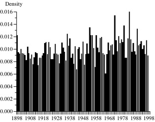
5. A researcher recorded annual precipitation in Rhode Island for 100 years, 1898-1997, and drew the histogram below by calculating density as the precipitation each year divided by the total precipitation for all 100 years. What is wrong with this histogram?
6. After Hurricane Katrina, Congress mandated that hurricane protection for New Orleans be improved to a 1-in-a-100 years standard, meaning that there is only a 1/100 probability of failing in any given year. Suppose you take out a 30-year mortgage in order to buy a home in this area. If the annual failure probability is 1/100 and, assuming independence, what is the probability of at least one failure in the next 30 years?
7. The overall unemployment rate of 10.2% in October 2009 was lower than the 10.8% unemployment rate in November 1982, which was the peak of the worst recession since the Great Depression. However, when the labor force was divided into four educational categories (college graduate, some college education, high-school graduate, and other), the unemployment rate in each category was higher in 2009 than in 1982! How is this possible? Be very specific. Don’t just say “the law of large numbers.”
8. A linear regression looked at the relationship between the dollar prices P of 45 used 2001 Audi A4 2.8L sedans with manual transmissions and the number of miles M the car had been driven:
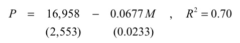
The standard errors are in parentheses. Be sure to explain your reasoning when you answer these questions:
a. Does the value 16,958 seem reasonable?
b. Does the value -0.0677 seem reasonable?
c. Is the estimated relationship between M and P statistically significant at the 5 percent level?
d. Should the variables be reversed, with M on the left hand side and P on the right hand side?
e. Suppose that the true relationship is P = α - β1M + β2C + ε, where C is the condition of the car and α, β1, and β2 are all positive. If M and C are negatively correlated, does the omission of C from the estimated equation bias the estimate of β1 upward or downward? Be sure to explain your reasoning.
9. A Yahoo sports story reported that in 2009, the Washington Redskins football team was the first team in NFL history to play 6 straight games against winless teams:
Week 1 -- New York Giants (0-0)
Week 2 -- St. Louis Rams(0-1)
Week 3 -- Detroit Lions (0-2)
Week 4 -- Tampa Bay Buccaneers (0-3)
Week 5 -- Carolina Panthers (0-3)
Week 6 -- Kansas City Chiefs (0-5)
The writer reported that the odds of this happening were 1 in 32,768, since 0.5^15 = 1/32,768. What is wrong with this calculation?
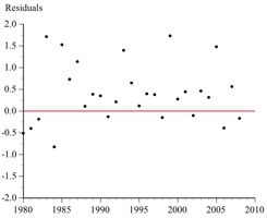
10. What is puzzling about this plot of the residuals from a least squares regression?
11. A study of major league baseball (MLB) managers from 1871 through 2007 found that 540 managers played professional baseball before becoming a manager, with the primary positions grouped as follows: pitcher (51), catcher (116), infielder (262), and outfielder (111). Use these data to test the null hypothesis that the respective probabilities are 1/9 pitcher, 1/9 catcher, 4/9 infielder, and 3/9 outfielder. What patterns do you see in your data? Are these patterns statistically persuasive?
12. In educational testing, a student’s ability is defined as the student’s (theoretical) average score on a large number of tests that are similar with respect to subject matter and difficulty. The student’s score on a particular test is equally likely to be above or below the student’s ability. Suppose that a group of 100 students takes two similar tests and the scores on each test have a mean of 65 with a standard deviation of 14. If a student’s score on the second test is 52, do you predict that this student’s score on the first test was: (a) below 52, (b) 52; (c) between 52 and 65; (d) 65; or (e) above 65? Explain your reasoning.
13. A study of a South India microfinance program estimated this least squares equation using 47 observations:
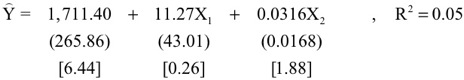
where Y = monthly family income, X1 = years in the microfinance loan program, and X2 = total amount loaned. The standard errors are in parentheses and the t-values are in brackets.
a. Is the coefficient of X2 substantial?
b. How was the t-value for the coefficient of X2 calculated?
c. How would you decide whether to calculate a 1-sided or 2-sided p-value for the coefficient of X2?
d. Explain why you either agree or disagree with this interpretation of the results: “The [one-sided] p-value for the total amount loaned is 0.032, which is not quite high enough to show that the amount loaned is statistically significant at the 5 percent level.
14. When a National Football League (NFL) game is tied at the end of regulation, the teams play a 15-minute sudden death overtime with a coin flip used to decide which team kicks off and which team receives. The first team to score wins. During the 2001-2006 seasons, there were 109 sudden death overtime games, one of which was still tied at the end of the overtime period because neither team scored. In the other 108 games, the team that received the ball first won 64 games and the team that kicked off won 44 games. Use these data to calculate the exact two-sided p value for a test of the null hypothesis that of those games decided by sudden death overtime, the kicking and receiving teams have an equal chance of winning.
15. A researcher asked 100 college students, “Aside from the obvious gender differences, do you most resemble your biological mother or father?” Identify several errors in this description of the statistical test:
The following equation is the basis for the Z-score I obtained:
The p-value is the area under the curve outside of two standard deviations of the mean.
16. A student reported taking a random sample of size 1000 from a population of 10,000 containing 4,000 women and 6,000 men, and obtaining 402 women. If this was a random sample, what is the probability that the sample proportion would be so close to 40%? Use a normal approximation.
17. A researcher compared the daily returns from a portfolio consisting of stocks that had been deleted from the Dow Jones Industrial Average with a portfolio consisting of the stocks that replaced them. Use these data for a difference-in-means test. What is the null hypothesis?
Deletion Portfolio Return |
Addition Portfolio Return |
Difference in Return |
|
| Mean | 0.000588 |
0.000433 |
0.000155 |
| Standard deviation | 0.012444 |
0.011862 |
0.008344 |
| Number of observations | 20,367 |
20,367 |
20,367 |
18. Use the data in Exercise 17 to do a matched-pair test. How can a matched-pair test give a different p-value than a difference-in-means test? Don’t just show formulas. Explain to someone who hasn’t studied statistics.
19. If you use the data summarized in Exercise 17 for an ANOVA test, how will the F value and p value be related to your answers to Exercises 17 and 18?
20. A multiple-choice test has 60 questions, each with 5 possible answers: a, b, c, d, e. Each question receives a score of 0 if it is left blank, +1 if it is answered correctly, and X if it is answered incorrectly.
a. What value of X would make the expected value of the score equal to zero for someone who randomly selects an answer? Show your work.
b. If the test administrator uses the value of X you derived in Part (a), and a student encounters a question where she has a probability P of answering the question correctly, for what values of P does answering this question give her a positive expected value on this question? Show your work.

