a. 5
b. 4
c. 3
d. 14
e. 12
f. 6
2. Survivor bias. We are ignoring the companies that are no longer around and also grouping companies by their current size, rather than their initial size. We should separate companies into quintiles based on their size 20 years ago.
3.
a. There is self-selection bias here in that the students who choose to go to Eastern Michigan may know that they would have trouble graduating from the University of Michigan. We also don’t know whether these students who could have attended the University of Michigan are among the 39% who did graduate from Eastern Michigan.
b. We would have to do a controlled experiment in which students who are admitted to the University of Michigan and Eastern Michigan are randomly assigned to each university; we could then compare their graduation rates.
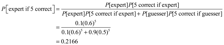
4. Using Bayes’ Rule,
Using a contingency table with 1,000 advisers:
5 correct |
not 5 correct |
total |
||||
| expert | 100*0.6^5 |
100 - 100*0.6^5 |
100 |
|||
| guesser | 900*0.5^5 |
900 - 900*0.5^5 |
900 |
|||
| total | 100*0.6^5 + 900*0.5^5 |
1,000 - (100*0.6^5 + 900*0.5^5) |
1,000 |
The probability that a person who gets 5 out of 5 correct is an expert is 100*0.6^5/(100*0.6^5 + 900*0.5^5) = 0.2166
5. For a histogram, we should group the 100 annual observations into a small number of categories, such as 0-10 inches, 10-20 inches, and so on. The density is the fraction of the total number of years with rainfall in that interval, divided by the interval width.
6. Using the subtraction rule,
![]()
7. Simpson’s Paradox. Unemployment rates are lower among more highly educated workers, and there were more highly educated workers in 2009 than in 1982.
8.
a. 16,958 is the predicted price if the car has never been driven. This value seems reasonable.
b. This equation predicts that driving an extra mile reduces the price of the car by 0.0677, about 7 cents/mile. This seems reasonable.
c. The estimated relationship between M and P statistically significant at the 5 percent level because the t-value is much larger than 2: t = -0.0677/0.0233 = 2.91.
d. No, mileage affects price; price does not affect mileage.
e. The estimate of β1 will be biased upward. When M goes up, C tends to go down, which reduces the price. Therefore an increase in M will seem to have a larger negative effect on price.
9. He calculated the probability that these teams would lose 15 games, assuming each team has a 0.5 probability of winning each game. The Redskins seem to have a favorable schedule in that they played several bad teams. A team that is 0-5 probably does not have a 0.5 probability of winning each game. The 15 is also wrong because the team they play in week 1 hasn't played a game yet.
10. The average value of the residuals is not equal to zero.
11.The observed and expected values are
Observed |
Expected |
|||
| pitcher | 51 |
60 |
||
| catcher | 116 |
60 |
||
| infielder | 262 |
240 |
||
| outfielder | 111 |
180 |
Catchers are greatly overrepresented; outfielders are greatly underrepresented. The chi-square value is 82.083, with a p-value less than 1.0 x10^-10.
12. Regression to the mean teaches us that this student’s ability is probably below average, but not as far below average as was this test score. The score on the second test is most likely between 52 and 65.
13.
a. The 0.0316 coefficient of X2 implies that a $1 loan increases annual income by 12*0.03 = 0.36, which seems substantial.
b. The t-value is equal to the value of the estimated coefficient divided by the standard error: 0.0316/0.0168 = 1.88.
c. I would only use a 1-sided p-value for the coefficient of X2 if I was certain before doing the study that a loan would not reduce income.
d. We want a low p value, not a high one. The two-sided p value is 0.064, not quite low enough to show statistical significance at the 5 percent level.
14. The exact binomial probability is
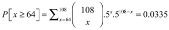
The two-sided p value is 2(0.0335) = 0.0670.
15. The null hypothesis should be that the success probability is 0.5, not the value of some population mean. If it were a test about the population mean, the Z statistic would look at the sample mean and the standard deviation of the sample mean

The p-value is the area under the normal curve that is outside of the observed Z-value.
16. We use a normal approximation to the binomial distribution. If p = 0.40, then the probability that x will be between 398 and 402 is
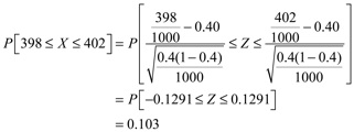
(The exact binomial probability is 0.128)
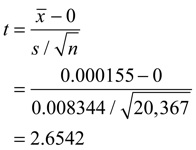
17. The value of the t-statistic is
The 2-sided p-value is 0.1977. The null hypothesis is that the population means are equal.
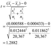
18. The value of the t-statistic is
The 2-sided p-value is 0.0080. A difference-in-means test assumes two independent random samples and has to take into account the possibility that, by the luck of the draw, the deletion portfolio returns might have occurred during a period in which the stock market was doing relatively well and the addition portfolio returns might have occurred during a period in which the stock market was doing relatively poorly. This possibility is controlled for in a matched-pair test because both time periods are exactly the same.
19.With two samples, an F-test is equivalent to a difference-in-means test
a. The ANOVA F-value is equal to the squared value of t in Exercise 17.
b. The ANOVA p-value is equal to two two-sided p-value in Exercise 17.
20. The expected value is the probabilty-weighted average of the possible outcomes.
a. A random answer has a 1/5 probability of being correct and a 4/5 probability of being incorrect, giving an expected value of E[X] = 1(1/5) + X(4/5) = 0 if X = -1/4.
b. If X = -1/4, the expected value is E[X] = 1(P) + (-1/4)(1 - P) = 5/4P - 1/4 > 0 if P > 1/5.
