2. Arranging the 30 observations in order,
| 34.04 | 30.57 | 26.81 | 26.33 | 26.32 | 23.66 | 18.00 | 17.45 | 17.00 | 16.69 |
| 16.54 | 15.37 | 14.97 | 14.41 | 12.91 | 12.31 | 11.01 | 10.92 | 10.70 | 9.98 |
| 9.26 | 9.11 | 8.92 | 8.90 | 7.98 | 7.58 | 6.54 | 6.49 | 5.83 | 4.56 |
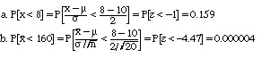
Here are the observed frequencies and histogram heights:
| Interval | Number | Histogram Height |
| 0-9.99 | 11 | 11/10 = 1.1 |
| 10-14.99 | 7 | 7/5 = 1.4 |
| 15-19.99 | 6 | 6/5 = 1.2 |
| 20-34.99 | 6 | 6/15 = 0.4 |
Here is a histogram:
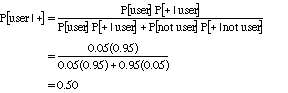
3. We can use a contingency table as in the textbook, assuming that a population of 10,000 people are tested:
| Test Positive | Test Negative | Total | |
| Drug-user | 475 | 25 | 500 |
| Drug-free | 475 | 9,025 | 9,500 |
| Total | 950 | 9,050 | 10,000 |
Thus P[drug-free | positive reading] = 475/950 = 0.50
Or we can use Bayes' theorem:
4. It doesn't matter! Let R be the number of red and blue marbles in the first can, with 50 - R marbles in the second can. Because you have an 0.5 probability of selecting each can, your overall probability of picking a red marble is
(This problem is much trickier if you don't have to have fifty marbles in each can; then your best strategy is to put one red marble and no blue marbles in one can and all the rest in the other can, giving you a 0.5 + 49/99 probability of winning.)
5. Marilyn arrived at the correct answer (A) by listing all the possibilities, but we can calculate the probabilities directly. The probability of no aces is equal to the probability that the first card is not an ace multiplied by the probability that the second card is not an ace, given that the first card is not an ace: (4/6)(3/5) = 0.40. The probability of one or both aces is 1 minus the probability of no aces: 1 - 0.40 = 0.60.
6. a. The R-squared is relatively low (the equation is not a perfect predictor), but the t value for x1 is large enough to provide statistically persuasive evidence that high-school GPA is a helpful predictor of a student's grade in this chemistry course.
b. The coefficient of x1 is biased downwards. Students who have taken a high school chemistry course tend to have relatively low high school GPAs and do well in a college chemistry course. If we omit x3, it will seem that students with low high school GPAs tend to do well in a college chemistry course and that students with better-than-average high school GPAs tend to do poorly in a college chemistry course.
7. a. Actually, 74 percent of the variation in heights.
b. The coefficient of x1 shows that, for given parental heights, a male is predicted to be 0.434 feet taller than a female. The t value merely tells us whether we can reject the null hypothesis that there is no difference between males and females, not the direction or size of the difference,
c. Yes, a student whose parents are each one-foot above average is predicted to be only 0.364 + 0.456 = 0.820 feet above average.
8. a. The first equation only allow the intercepts to differ, so that each nonfiction book costs 29 cents more than a fiction book with the same number of pages; for each category, the price rises by 2.2 cents per page. The second model is richer in that it allows the intercept and the slope to differ.
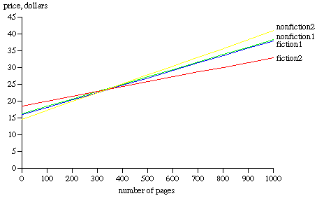
b. Plugging in the values y = 18.49 + 0.0144(300) - 3.90((1) + 0.0119(300)(1) = $22.48
c. The t value is (0.0144 - 0.05)/0.0053 = 6.72; there are 30 - 4 degrees of freedom and the two-sided p value is minuscule. The alternative hypothesis is that the coefficient is not equal to 0.05.
9. a. Using a difference-in-proportions test (and the fact that 0.41(81) = 33 and 0.11(81) = 9,
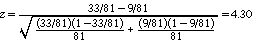
The two-sided p value is 0.000008. b.
Perhaps the exposure to hardened criminals had not scared the participants, but instead motivated them to imitate the prisoners' attitudes.
10. For the three categories (corner, adjacent, and other), 3/15 of the balls are in the corners, 6/15 are adjacent, and 6/15 are other, implying these expected values:
| Observed | Expected | ||
| Corner | 25 | (3/15)(54) = 10.8 | |
| Adjacent | 22 | (6/15)(54) = 21.6 | |
| Other | 7 | (6/15)(54) = 21.6 | |
| Total | 54 | 54 |
Far more corner balls were sunk and far fewer in the other category than would be expected if each ball were equally like to be sunk. The chi-square value is 28.55,
which decisively rejects the null hypothesis, since Table 6 in the textbook shows that, with 3 - 1 = 2 degrees of freedom, the cutoffs are 5.99 for a test at the 5 percent level and 9.21 for a test at the 1 percent level. (Statistical software shows that the P value is 0.0000007.)
11. If x is normally distributed with a mean of 68 and a standard deviation of 3, then the mean of a random sample of four observations is normally distributed with a mean of 68 and a standard deviation of 3 divided by the square root of 4. which is 1.5. Table 3 in the textbook shows that there is a 0.01 probability that a normally distributed random variable will be 2.575 standard deviations away from its mean. Therefore, the appropriate upper and lower control limits are
12. The null hypothesis is that each volunteer is equally likely to show an increase or decrease in strength; that is, that the probability of showing a decrease in strength is 0.5. Using the binomial distribution with n = 10 and p = 0.5, the probability of 7 or more successes is 0.1719:
Therefore, if we use 7 or more for the cutoff in a one-tailed test of the null hypothesis, then the probability of rejecting the null hypothesis when it is true is 0.1719.
13. The differences among the sample means, particularly between cars A and B, seem large compared to the variation within each sample. (The P value is in fact less than 0.05.) The null hypothesis is that the populations from which these three samples came all have the same mean.
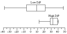
14. The box plots show the high D/P stocks to generally have higher returns than the low D/P stocks and to have considerably less variation in the returns (we shouldn't assume the population standard deviations to be equal!):
Here are the sample means and standard deviations:
| High D/P | Low D/P | |
| Mean | 30.96 | 8.09 |
| Standard deviation | 10.24 | 28.35 |
These calculations confirm the visual impression in the box plots: the high D/P stocks did much better, on average, than the low D/P stocks, and with considerably less dispersion in the returns. The t value for a difference in means test is 2.399:
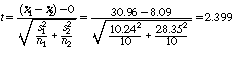
Statistical software shows that there are 11.3 degrees of freedom and P[t > 2.399] = 0.0174, giving a two-sided P value of 2(0.0174) = 0.0348. The observed differences in the mean returns is substantial and barely statistically significant at the 5 percent level.
15. Transforming to standardized z values: