Econ 57 Spring 1999 Final Examination Answers
1. A chi-square test with expected values of 370/7 for each day gives a chi-square value of 35.159; with 7 - 1 = 6 degrees of freedom, the p value is 0.000004.
2. For H0: p = 0.5, the exact binomial probability of 51 or more successes in 99 trials is 0.41, giving a two-sided p value of 0.82. For a normal approximation, the z-value is
3. Self-selection bias. There may be systematic differences in the mathematical abilities of those who choose to major in economics and in other fields. We don't know if their test scores reflect these differences or their study of economics.
4. Relative to the sample sizes and standard deviations, the mean of sample1 seems quite far from the other two means. The P value is surely less than 0.05, so that this difference is statistically significant at the 5 percent level. (The F value is 8.33 and the P value is 0.00005.)
5. a. Because weather may influence people's clothing, but not the other way around, the student correctly chose clothing to be the dependent variable.
b. The positive estimated coefficient for x indicates that the sunnier the day, the brighter the clothing.
c. The t value for the coefficient of x is 0.423/0.092 = 4.60, high enough to make the relationship statistically significant at the 5 percent level. (The cutoff for a two-tailed test with 11 degrees of freedom is 2.201.)
d. There is considerable ambiguity in classifying both the weather and clothing brightness. Is dark-red clothing brighter than light-brown? What about clothing that contains more than one color?
6. An increase in the numerical value of the ranking (from 10 to 20, for instance) signifies a drop in the U.S News rankings, and should, if anything, reduce the number of applications. Thus we expect a negative relationship.
The division of each value by 1.04 does not adjust for an annual growth of
4 percent, but merely makes each value 4 percent smaller. If the number of applicants
increases by 4 percent a year, we need to divide the 1988 unadjusted value by
1.04, the 1989 unadjusted value by 1.042, and so on. Growing by 4 percent a
year, the total number of applications nationwide is 36.9 percent higher in
1995 than in 1987 (1.048 = 1.369), and we consequently need to divided the unadjusted
1995 value by 1.369. Here are the correct calculations:
| Number of Applications | ||
| Unadjusted | Adjusted | |
| 1987 | 3192 | 3192.0 |
| 1988 | 2945 | 2945/1.04 = 2831.7 |
| 1989 | 3176 | 3176/1.042 = 2936.4 |
| 1990 | 2869 | 2869/1.043 = 2550.5 |
| 1991 | 2852 | 2852/1.044 = 2437.9 |
| 1992 | 2883 | 2883/1.045 = 2369.6 |
| 1993 | 3037 | 3037/1.046 = 2400.2 |
| 1994 | 3293 | 3293/1.047 = 2502.4 |
| 1995 | 3586 | 3586/1.048 = 2620.3 |
7. The difference between 8.7 percent and 5.4 percent does seem substantial. Not rejecting the null hypothesis does not prove the null hypothesis to be true. The small sample size is taken into account in the standard deviation calculation for the z statistics and does not invalidate her results.
8. There would have been no effect, because the fitted line that minimizes the sum of squared prediction errors does not depend on the ordering of the data.
9. We need equal sample sizes only for regression, where we must pair the x and y values.
10. The difference in the heart attack rates (4/412 = 0.0097 versus 17/358 = 0.04749) does seem substantial; those on the low-fat diet were nearly five times more likely to experience a second heart attack. For a statistical test, the pooled proportion is (4 + 17)/(412 + 358) = 0.02727, and the z value is
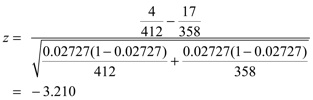
The two-sided p value is 0.001. A chi-square test can also be used (and gives the same p value.).
11. The intercept a is the salary of a male with no teaching experience; b1 is the difference between female and male salaries at every experience level (a + b1 is the salary of a female with no teaching experience); b2 is the increase in male salaries for each additional year of experience; b3 is the difference between female and male salary increases for each additional year of experience (b2 + b3 is the increase in female salaries for each additional year of experience).
a. A difference-in-means test doesn't take experience into account.
b. Suppose that salaries rise with experience. If there is no discrimination and males happen to have more experience than females, a regression equation can show no discrimination while a difference-in-means test does. (Similarly, if there is discrimination and males happen to have less experience than females, a regression equation can show discrimination while a difference-in-means test does not.)
12. These can all be determined using the subtraction rule and the binomial distribution:
a. 1 - (5/6)6 = 0.6651
b. 1 - (5/6)12 - 12(1/6)(5/6)11 = 0.6187
c. 1 - (5/6)18- 18(1/6)(5/6)17 - {18(17)/2}(1/6)(1/6)(5/6)16 = 0.5973
Logically, Part a is 1 minus the probability that all six of the dice are not 6s. Part b is 1 minus the probability that either all twelve dice are not 6s or that exactly one of the twelve dice is a 6; this latter probability is as written because there are 12 sequences for rolling a 6 on one die and a non-6 on the other 11 dice. Part c is 1 minus the probability of no 6s, exactly one 6, or exactly two 6s. There is one sequence of non-6s, 18 sequences of one 6 and seventeen non-6s, and (18)(17)/2 sequences of two 6s and sixteen non-6s.
13. The number of pages haven't been adjusted for the size of the yellow pages and hence the size of the cities. (These same researchers found that personal bankruptcy rates tend to be higher in large cities than in smaller ones.) Also, the selection of 7 cities for one group and 5 for the other sounds like data mining. Perhaps most importantly, the causation may run the other way around: cities with lots of personal bankruptcy filings tend to encourage bankruptcy lawyers to set up practices.
14. This probability can be calculated from a contingency table. To simplify calculations with the one-third WSI, assume a total population of 300. Of these, 100 (one third) have a woman as the sole income provider and 45 (15 percent) are poor. Of the 45 households that are poor, 27 (60 percent) have a woman as the sole income provider. The remaining numbers in the table can be filled in from these data.
| WSI | Not WSI | Total | |
| Poor | 27 | 18 | 45 |
| Not poor | 73 | 182 | 255 |
| Total | 100 | 200 | 300 |
15. The 0.20 difference in average GPAs is not trivial, but isn't very large either. For statistical significance, a difference-in-means test gives a t value of 2.510 and, with 25.3 degrees of freedom, a two-sided P value of 0.019
16. a. The null hypothesis is that the contents of a bag of plain M&M's constitute a random sample from a population with the candy colors distributed according to the manufacturer's claims. Thus each M&M has a 30 percent chance of being brown, a 20 percent chance of being red, and so on.
b. The error in their calculation is that they should have used the number of observed and expected M&M's, not the percentages.
c. Logically, their statistic is flawed because it does not reflect the number of M&M's in the sample. For example, these could be 34 and 30 percent of 100 M&M's or 100,000 M&M's. The observed 4-percentage-point difference is more persuasive evidence against the null hypothesis when the sample size is large.
17. These are not two independent observations, as required by a random sample, but rather the upper and lower limits on a single observation.
18. The z value and normal probability are:
19. The units on the horizontal axis are inconsistent, ranging from 8 months to 5 years. They should have deflated the data by the price level in each year, in order to show the how the real cost has changed over time. (In fact, a note at the bottom of the table states that "In 1971 dollars, the price of a 32-cent stamp in February 1995 would be 8.4 cents," a peculiar note since the article appeared in March of 1994.]
20. The logic underlying the regression-toward-the-mean phenomenon suggests that he is the tallest. The height of someone who is very tall is probably an overstatement of this person's genetically inherited height--which is the genetically inherited height of the brothers.
