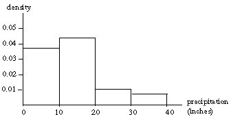
2.7 Arranging the 30 observations in order:
| 34.04 | 30.57 | 26.81 | 26.33 | 26.32 | 23.66 | 18.00 | 17.45 | 17.00 | 16.69 |
| 16.54 | 15.37 | 14.97 | 14.41 | 12.91 | 12.31 | 11.01 | 10.92 | 10.70 | 9.98 |
| 9.26 | 9.11 | 8.92 | 8.90 | 7.98 | 7.58 | 6.54 | 6.49 | 5.83 | 4.56 |
Here are the observed relative frequencies and the histogram heights (the
relative frequencies divided by the interval widths). Because the interval widths
are equally wide, the histogram looks the same as a bar chart, but has different
units on the vertical axis.
| Interval | Number | Relative Frequency | Histogram Height | |||
| 0-9.99 | 11 | 11/30 = 0.367 | 0.367/10 = 0.0367 | |||
| 10-19.99 | 13 | 13/30 = 0.433 | 0.433/10 = 0.0433 | |||
| 20-29.99 | 4 | 4/30 = 0.133 | 0.133/10 = 0.0133 | |||
| 30-39.99 | 2 | 2/30 = 0.067 | 0.067/10 = 0.0067 | |||
| Total | 30 | 1.000 |
Here is a histogram:
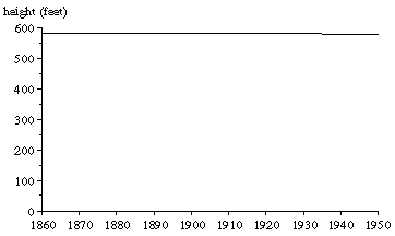
2.14 Here is the graph with the vertical axis going from 0 to 600:
Here is graph with the vertical axis going from 579 to 584:
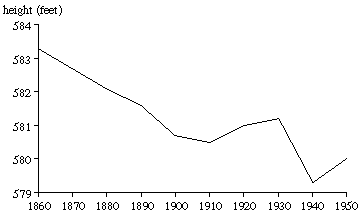
The graph with the vertical axis going down to zero puts the decline into perspective (less than a 1 percent drop), but is otherwise useless: we can hardly tell that there has been a decline and certainly can't see the fluctuations in the data (including the rise between 1910 and 1930). In the graph with zero omitted, we can clearly see the decline and the fluctuations, but we should not let the steepness of the figure mislead us about the magnitude of the decline. We have to look at the actual data to see that over this 100-year period, the height of Lake Michigan has declined by 3.3 feet, an average of about half an inch per year.
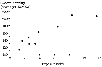
2.18 The exposure index is the explanatory variable and cancer mortality is the dependent variable since exposure to radioactive wastes may cause cancer, but not vice versa. A scatter diagram shows a positive relationship:
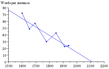
2.26 The extension of a line fit to these data for 1598 to 1940 indicates negative words per sentence in the year 2200! This incautious extrapolation is clearly too ridiculous to be taken seriously. (In Chapter 11, we will see how to fit a line to the data by ordinary least squares; the equation for this line is y = 264.81 - 0.125x, which implies y = 264.81 - 0.125(2200) = -10.19 in the year 2200.)
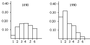
2.34 Here are the relative frequencies:
| Households in 1890 | Households in 1990 | |||
| Size | Number | Relative Frequency | Number | Relative Frequency |
| 1 | 0.457 | 0.457/12.690 = 0.036 | 23.0 | 23.0/93.8 = 0.245 |
| 2 | 1.675 | 1.675/12.690 = 0.132 | 30.2 | 30.2/93.8 = 0.322 |
| 3 | 2.119 | 2.119/12.690 = 0.167 | 16.1 | 16.1/93.8 = 0.172 |
| 4 | 2.132 | 2.132/12.690 = 0.168 | 14.6 | 14.6/93.8 = 0.156 |
| 5 | 1.916 | 1.916/12.690 = 0.151 | 6.2 | 6.2/93.8 = 0.066 |
| 6 | 1.472 | 1.472/12.690 = 0.116 | 2.2 | 2.2/93.8 = 0.023 |
| 7-10 | 2.919 | 2.919/12.690 = 0.230 | 1.5 | 1.5/93.8 = 0.016 |
| Total | 12.690 | 1.0000 | 93.8 | 1.0000 |