(2)
Do Baseball Players Regress Toward the Mean?
Edward M. Schall
Andersen Consulting
San Francisco, California
94105
Gary Smith
Department of Economics
Pomona College
Claremont, California 91711
gsmith@pomona.edu
Edward M. Schall is a Business Analyst at Andersen Consulting, San Francisco, CA 94105 (E-mail: tms@sirius.com); Gary Smith is Fletcher Jones Professor of Economics, Pomona College, Claremont, CA 91711 (E-mail: gsmith@pomona.edu). The authors thank the referees for their careful reading and very helpful comments.
Abstract
Baseball performances are an imperfect measure of baseball abilities, and consequently exaggerate differences in abilities. Predictions of relative batting averages and earned run averages can be improved substantially by using correlation coefficients estimated from earlier seasons to shrink performances toward the mean.
key words: least squares, sports, predictions
Do Baseball Players Regress Toward the Mean?
1. INTRODUCTION
Baseball players who win coveted awards and sign breathtaking contracts often disappoint fans, managers, and owners. These disappointments might be explained by regression toward the mean, which occurs when real phenomena are measured imperfectly, causing extreme measurements to exaggerate differences among the underlying phenomena. The degree of exaggeration depends on the correlation between the measurements and the real phenomena. In baseball, the correlation between performance and skill is far from perfect and, as a consequence, observed performance differences substantially overstate skill differences. Players who do exceptionally well in any particular season typically do not do as well the subsequent season–they regress toward the mean. We can improve our forecasts by adjusting our predictions accordingly.
2. REGRESSION TOWARD THE MEAN
Galton (1886) observed regression toward the mean in his seminal study of the relationship between the heights of parents and their adult children. Because heights are affected by diet, exercise, and other environmental factors, observed heights are an imperfect measure of the genetic influences that we inherit from our parents and pass on to our children. A person who is 78 inches tall may have been pulled above a somewhat shorter genetically predicted height by positive environmental influences or may have been pulled below a somewhat taller genetic height by negative environmental factors. The former is more likely because there are many more people with genetically predicted heights below 78 inches than with genetic heights above 78 inches. Thus the observed heights of unusually tall parents usually overstate the genetic heights that they pass on to their children.
Regression toward the mean can be seen in sports, where observed performance is an imperfect measure of skill. Of the last twenty major league baseball champions from 1979 through 1998, only two repeated the following year. Of those major league baseball teams that win more than 100 games in a season, 90% do not do as well the next season (James 1981). Outcomes depend on luck as well as skill, and those teams that do unusually well are more likely to have experienced good luck than bad. Few teams are so far superior to their opponents that they can win a championship in an off year. Thus the performance of most champions exaggerates their skill and, because good luck cannot be counted on repeatedly, most champions regress to the mean.
The same is true of individual players. In 1989, Sports Illustrated reported that of those baseball players who hit more than 20 home runs in the first half of the season, 90% hit fewer than 20 during the second half. The writer concluded that there was a "second-half power outage" (Gammons 1989, p. 68). The regression-toward-the-mean explanation is that their skills did not deteriorate, but rather that their unusually good performances during the first half exaggerated their skills. Regression toward the mean can also explain such cliches as the Cy Young jinx, sophomore slump, rookie-of-the-year jinx, and Sports Illustrated cover jinx. Baseball players have good and bad years, and it would be extraordinary for a player to be the best in the league while having a bad year by his own standards. Most players who do much better than their peers are also performing better than their own career averages.
Tables 1 and 2 show the players who had the ten best batting averages (BAs) and earned-run averages (ERAs) in 1998 among those players who had at least 50 at bats or 25 innings pitched in 1997, 1998, and 1999. The mean batting average was approximately 30 points lower in the adjacent seasons than in the top-10 season; the mean earned run average was roughly 1 run higher. Thirteen of these twenty players had worse records in both 1997 and 1999 than in 1998.
More generally, Figures 1 and 2 compare the 1998 and 1999 BAs and ERAs of all major league players who had at least 50 at bats or 25 innings pitched in each of these years. (These figures also show the locally weighted scatter plot smoothing (LOWESS) lines with a bandwidth of 0.5. Ramsey regression specification error tests for second-, third-, or fourth-order terms have p values of 0.305 for batting averages and 0.172 for earned run averages.)
These graphs have two striking characteristics. First, although the relationships are highly statistically significant, the correlations are modest. For the 381 batters, the two-sided p value is 95.3 x 10—13 and the correlation coefficient is 0.36; for the 300 pitchers, the two-sided p value is 0.00000004 and the correlation coefficient is 0.31. Although the 1998 performances are statistically helpful in predicting 1999 performance, the predictions are far from perfect.
Second, the slopes of the least-squares lines are less than 1, indicating that performance regresses to the mean. Because the least-squares line goes through the average values of both variables, the 0.378 slope for batters means that a player whose BA was 0.050 above (or below) the 1998 mean is predicted to have a 1999 batting average that is only 0.019 from the 1999 mean. The 0.340 slope for pitchers implies that a player whose ERA was 1.000 from the 1998 mean ERA is predicted to have a 1999 ERA that is only 0.340 from the 1998 mean.
For another suggestive indicator of regression toward the mean, we looked at all major league players since 1901 who had at least 50 at bats or 25 innings pitched in two consecutive seasons. Of 4026 players who had BAs of .300 or higher in any season, 3210 (79.7%) did worse the following season. Of 3849 players who had ERAs of 3.00 or lower in any season, 3077 (79.9%) did worse the following season. Clearly, baseball players regress toward the mean. To formalize these observations, we use the following model.
3. A MODEL
Let Y be a statistical measure of a player’s performance (batting average for batters, earned run average for pitchers). In order to compare players from different seasons, we standardize performance by taking the difference between the player’s performance in any given season and the mean performance for all players that season, and dividing this difference by the standard deviation of performance across players that season. Thus Ted Williams’ .406 batting average in 1941 was a standardized batting average of Z = 3.14; that is, 3.14 standard deviations above the mean that year. Sandy Koufax’s 1.73 earned run average in 1966 was standardized to be Z = –1.93, or 1.93 standard deviations lower than the mean ERA that year.
A player’s performance Z in any year is related to an expected value m, which we can think of as this player’s true ability (what his average performance would be over many similar seasons). The player’s actual performance in any particular season differs from his ability by a random term e that we assume has an expected value of zero and is independent of ability and of the value of the random term in other seasons:
|
Z = m
+ e
|
(1)
|
There is a distribution of abilities across players. If e is independent of m, then the variance of Z is equal to the variance of m plus the variance of e, and is therefore larger than the variance of m: var[Z] = var[m] + var[e]. Thus the variation of actual batting averages (or earned run averages) across players in a season is larger than the variation of abilities. An extreme performance typically overstates how far this player’s ability is from the mean ability.
If we knew the value of a player’s ability m, we could use m to make an unbiased prediction of his performance in a season. However, players, fans, managers, and owners are interested in the reverse question–using performance to predict ability–and unbiased predictions require an adjustment for regression toward the mean.
Imagine that we had data on each person’s ability m and his performance Z in a season. The least-squares equation for predicting performance from ability is
|
|
(2)
|
where r is the correlation between
Z and m. The least-squares equation for predicting
ability from performance is
|
|
(3)
|
Unless the correlation coefficient is 1 or –1, these two equations are not simply the reverse of each other.
Because they cannot use the unknown value of m to predict performance Z in any given season, fans, managers, and owners might use the value Z(–1) in the preceding season:
Z = a + bZ(–1) + g
Using Equation 1 and assuming abilities are constant in adjacent seasons, the true relationship is
Z = Z(–1) + (e – e(–1))
If var[e(–1)] = var[e], then the correlation coefficient between Z and Z(–1) is a simple function of the variation in abilities and the variation in performance about ability:
![]()
The greater the variation in performance about abilities, the smaller is the correlation between adjacent-season performances and the more we should shrink predicted performances toward the mean.
4. DATA
We looked at season batting averages and earned run averages for all major league baseball batters and pitchers from 1901 through 1999 (Thorn, et al, 1999). To reduce the influence of outliers, we excluded players who had fewer than 50 official times at bat or 25 innings pitched. This gave us a database of 29,310 seasons for 5262 batters and 20,385 seasons for 4212 pitchers. To compare players from different years, each player’s performance each year was standardized by subtracting the mean for all players that year and dividing this difference by the standard deviation of performance across players that year. In addition, in a competitive sport like baseball, relative performance is what matters–not whether a player bats .290, but how many standard deviations the player is above or below the mean that year.
5. PERFORMANCE CORRELATIONS
We calculated correlation coefficients in two ways. For the most-recent-season calculation, we compared a player’s performance in a given year with his performance in the most recent preceding season; for the more restrictive adjacent-season comparison, we only considered cases where the most recent season immediately preceded the current season.
For batting averages, a total of 24,047 most-recent-season observations have a correlation coefficient of 0.37 and 22,243 adjacent-season observations have a correlation coefficient of 0.38. For earned run averages, a total of 16,172 most-recent-season observations have a correlation coefficient of 0.22 and 14,714 adjacent-season observations have a correlation coefficient of 0.24. In all cases, these correlations are highly statistically significant, decisively demonstrating that performance is not uncorrelated across seasons. However, the correlations are far from perfect.
These results are not an artifact of a few outliers who did extraordinarily well or poorly one season and more nearly average the next season. Excluding batters who were more than 2 standard deviations from the mean in the most recent or adjacent season, the correlation coefficients drop slightly, to 0.34 and 0.35. Excluding pitchers who were more than 2 standard deviations from the mean, the respective correlation coefficients remain 0.22 and 0.24.
Looking at individual seasons, the BA correlation coefficients for adjacent seasons ranged from 0.18 in 1991 and 0.25 in 1940 to 0.63 in 1906 and 0.59 in 1931; the average was 0.39. Since World War II, the highest correlation coefficient was 0.46 in 1957. The ERA correlation coefficients for adjacent seasons ranged from 0.00 in 1913 and 1948 to 0.55 in 1939 and 0.48 in 1932; the average was 0.25. Since World War II, the lowest correlation coefficient was 0.05 in 1981 and the highest was 0.38 in 1977.
6. PREDICTING RELATIVE PERFORMANCE
Our model suggests that instead of using this year’s relative performance to predict next season’s relative performance, more accurate predictions can be made by shrinking each player’s performance toward the mean; that is, predicting a player’s Z(+1) from rZ rather than Z. To see whether this is so, we considered batters and pitchers who played in two adjacent seasons, say 1998 and 1999. The unadjusted prediction of each player’s 1999 Z value is simply his 1998 Z value. For the adjusted predictions, we used the data for all persons who played in both 1997 and 1998 to estimate the correlation coefficient between adjacent-season performance; we then predicted the 1999 Z value of each person who played in 1998 and 1999 by multiplying his 1998 Z value by this correlation coefficient.
We did this for every season and measured the overall accuracy of the predictions by the root mean squared error (RMSE) each year and for the entire time period. The first rows of Tables 3 and 4 show these results. For both batters and pitchers, the RMSE was improved in every one of the 96 years by shrinking the performances toward the mean. For the entire time period, the RMSE was reduced 16% for batters and 18% for pitchers.
For those who have played more than one year, more accurate predictions might be expected from an averaging of these previous seasons’ performances. Our model suggests that these averages, too, should be shrunk towards the mean. To investigate this question, we considered batters and pitchers who had played in 2n adjacent seasons, using the average Z value for the n earlier years to predict the average Z value for the n subsequent years. For example, with n = 2, we looked at persons who had played in 1995, 1996, 1997, and 1998. The unadjusted prediction of each player’s average Z value for 1997 and 1998 is his average Z value for 1995 and 1996. For the adjusted predictions, we calculated the correlation coefficient between average 1993–1994 Z values and average 1995–1996 Z values for all persons who played these four seasons. We then predicted each player’s 1997–1998 Z by multiplying his 1995–1996 Z by this correlation coefficient. We only made predictions when data for at least 25 players were available for estimating the correlation coefficient. There were consequently no BA predictions for horizons longer than 7 years and no ERA predictions for horizons longer than 6 years.
Tables 3 and 4 show the results. As the horizon lengthened and the Z values were averaged over more seasons, there is typically an increase in the correlation coefficient and a decline in the RMSE. For every horizon, the predictions were substantially improved by shrinking each player’s relative performance toward the mean.
These results are robust with respect to the minimum number of at bats and innings pitched. Tables 5 and 6 show the predictive accuracy for next-season forecasts with the minimum number of at bats ranging from 50 to 400 and the minimum number of innings pitched ranging from 25 to 200. These increases in the minimum numbers raise the average correlation coefficient, but do not alter our conclusion that shrinkage gives more accurate predictions of relative performance.
At the suggestion of a referee, we also looked at this performance measure for batters: on base average plus slugging average, where a player’s on base average is the sum of his hits, bases on balls, and times hit by pitches divided by the sum of his times at bat, bases on balls, times hit by pitches, and sacrifice flies; a player’s slugging average is his total bases (one base for a single, two for a double, three for a triple, and four for a home run) divided by his times at bat. Table 7 shows that the correlations between performances in different years are somewhat higher, but that the results are otherwise very similar to those for batting averages.
7. CONCLUSION
Because baseball performances are an imperfect measure of underlying abilities, batting averages and earned run averages regress toward the mean. Outstanding performances exaggerate player skills and are typically followed by more mediocre performances. The average correlation coefficient for adjacent-season performance is 0.39 for batting averages and 0.25 for earned run averages. Predictions of standardized batting averages and earned run averages can be improved consistently and substantially by using correlation coefficients estimated from earlier seasons to shrink performances toward the mean.
References
Galton, F. (1886), "Regression Towards Mediocrity in Hereditary Stature," Journal of the Anthropological Institute, 15, 246–263.
Gammons, P. (1989), "Inside Baseball," Sports Illustrated, 103, 68.
James, B. (1981), "Esquire’s 1981 Baseball Forecast," Esquire, 95, 106–113.
Thorn, J., Gershman, M., Palmer, P. and Pietrusza, D. (eds.) (1999), Total Baseball, Sixth Edition, New York: Total Sports; the latest data are available on the web site www.baseball.com.
Table 1. How the Ten Players with the Highest BAs in 1997 Did in 1996 and 1998
| 1997 | 1998 | 1999 | |
| Larry Walker | .366 | .363 | .379 |
| John Olerud | .294 | .354 | .298 |
| Bernie Williams | .328 | .339 | .342 |
| Mo Vaughn | .315 | .337 | .281 |
| Eddie Perez | .215 | .336 | .249 |
| Dante Bichette | .308 | .331 | .298 |
| Albert Belle | .274 | .328 | .297 |
| Mike Piazza | .362 | .328 | .303 |
| Eric Davis | .304 | .327 | .257 |
| Jason Kendall | .294 | .327 | .332 |
| Average | .306 | .337 | .304 |
Table 2. How the Ten Players With the Lowest ERAs in 1997 Did in 1996 and 1998
| 1997 | 1998 | 1999 | ||
| Ugueth Urbina | 3.78 | 1.30 | 3.69 | |
| Trevor Hoffman | 2.66 | 1.48 | 2.14 | |
| Robb Nen | 3.89 | 1.52 | 3.98 | |
| Mike Jackson | 3.24 | 1.55 | 4.06 | |
| Graeme Lloyd | 3.31 | 1.67 | 3.63 | |
| Mariano Rivera | 1.88 | 1.91 | 1.83 | |
| John Wetteland | 1.94 | 2.03 | 3.68 | |
| Jeff Shaw | 2.38 | 2.12 | 2.78 | |
| Greg Maddux | 2.21 | 2.22 | 3.57 | |
| Kevin Brown | 2.69 | 2.38 | 3.00 | |
| Average | 2.80 | 1.82 | 3.24 | |
Table 3. Predicting Standardized Batting Average from Earlier Z and rZ
|
Years
|
Number of
|
Average
|
Years with Lower RMSE
|
Cumulative RMSE
|
||
|
Ahead
|
Predictions
|
Correlation
|
Z
|
rZ
|
Z
|
rZ
|
|
1
|
22,107
|
0.392
|
0
|
97
|
1.048
|
0.884
|
|
2
|
14,422
|
0.553
|
0
|
94
|
0.723
|
0.644
|
|
3
|
9,546
|
0.633
|
5
|
86
|
0.607
|
0.549
|
|
4
|
5,883
|
0.678
|
4
|
79
|
0.546
|
0.493
|
|
5
|
3,223
|
0.715
|
7
|
59
|
0.518
|
0.464
|
|
6
|
1,069
|
0.675
|
3
|
22
|
0.511
|
0.449
|
|
7
|
158
|
0.650
|
0
|
8
|
0.501
|
0.410
|
Table 4. Predicting Standardized Earned Run Average from Earlier Z and rZ
|
Years
|
Number of
|
Average
|
Years with Lower RMSE
|
Cumulative RMSE
|
||
|
Ahead
|
Predictions
|
Correlation
|
Z
|
rZ
|
Z
|
rZ
|
|
1
|
14,649
|
0.245
|
0
|
97
|
1.129
|
0.923
|
|
2
|
8,806
|
0.290
|
2
|
92
|
0.803
|
0.677
|
|
3
|
5,190
|
0.319
|
11
|
73
|
0.667
|
0.577
|
|
4
|
2,508
|
0.294
|
6
|
44
|
0.610
|
0.537
|
|
5
|
1,088
|
0.223
|
11
|
17
|
0.581
|
0.548
|
|
6
|
182
|
0.374
|
7
|
7
|
0.531
|
0.483
|
Table 5. Predicting Year-Ahead Standardized Batting Average
|
Times
|
Number of
|
Average
|
Years with Lower RMSE
|
Cumulative RMSE
|
||
|
at Bat
|
Predictions
|
Correlation
|
Z
|
rZ
|
Z
|
rZ
|
|
50
|
22,107
|
0.392
|
0
|
97
|
1.048
|
0.884
|
|
100
|
19,025
|
0.422
|
0
|
97
|
1.048
|
0.895
|
|
200
|
14,594
|
0.460
|
0
|
97
|
1.033
|
0.893
|
|
400
|
7,250
|
0.503
|
2
|
93
|
1.007
|
0.881
|
Table 6. Predicting Year-Ahead Standardized Earned Run Average
|
Innings
|
Number of
|
Average
|
Years with Lower RMSE
|
Cumulative RMSE
|
||
|
Pitched
|
Predictions
|
Correlation
|
Z
|
rZ
|
Z
|
rZ
|
|
25
|
14,649
|
0.245
|
0
|
97
|
1.129
|
0.923
|
|
50
|
12,159
|
0.269
|
0
|
97
|
1.139
|
0.945
|
|
100
|
7,540
|
0.297
|
0
|
97
|
1.134
|
0.937
|
|
200
|
1,798
|
0.317
|
4
|
55
|
1.158
|
0.968
|
Table 7. Predicting Standardized On Base Average Plus Slugging Average
|
Years
|
Number of
|
Average
|
Years with Lower RMSE
|
Cumulative RMSE
|
||
|
Ahead
|
Predictions
|
Correlation
|
Z
|
rZ
|
Z
|
rZ
|
|
1
|
22,107
|
0.555
|
0
|
97
|
0.926
|
0.822
|
|
2
|
14,422
|
0.696
|
4
|
90
|
0.667
|
0.617
|
|
3
|
9,546
|
0.745
|
10
|
81
|
0.586
|
0.547
|
|
4
|
5,883
|
0.773
|
5
|
78
|
0.548
|
0.511
|
|
5
|
3,223
|
0.790
|
8
|
58
|
0.541
|
0.501
|
|
6
|
1,069
|
0.746
|
1
|
24
|
0.547
|
0.495
|
|
7
|
158
|
0.659
|
2
|
6
|
0.515
|
0.453
|
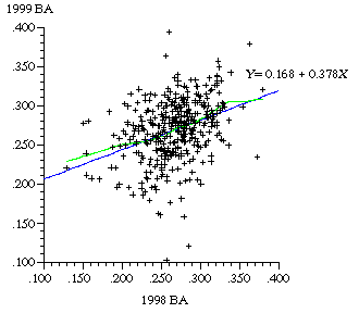
Figure 1. 1998 and 1999 Batting Averages
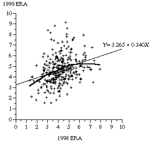
Figure 2. 1998 and 1999 Earned Run Averages