Shrunken Earnings Predictions are Better Predictions

Margaret H. Smith, Pomona College
Manfred Keil, Claremont McKenna College
Gary Smith, Pomona College

Abstract

Analysts’ earnings forecasts are not perfectly correlated with actual earnings. One statistical consequence is that the most optimistic and most pessimistic forecasts are usually too optimistic and too pessimistic. The forecasts’ accuracy can be improved by shrinking them toward the mean. Insufficient appreciation of this statistical principle may partly explain the success of contrarian investment strategies, in particular why stocks with the most optimistic earnings forecasts underperform those with the most pessimistic forecasts.

key words: earnings forecasts, regression to the mean, contrarian investment strategies

This research was supported by the TIAA-CREF Institute.

Shrunken Earnings Predictions are Better Predictions

Predicted earnings are not perfectly correlated with actual earnings. One consequence is that the largest predicted earnings growth rates are more likely to be excessively optimistic predictions than to be overly pessimistic. Similarly, the lowest predicted growth rates are more likely to be too pessimistic than too optimistic. If so, the adjustment of stock prices when earnings turn out to be closer to the mean than was predicted may partly explain the success of contrarian strategies.

This paper’s objective is to see whether the statistical principle of regression toward the mean can be used to improve analysts’ forecasts of earnings growth rates. Section 1 gives a brief overview of the literature on contrarian strategies. Sections 2 and 3 focus on regression toward the mean and its implications. Section 4 presents our forecasting model, Sections 5 and 6 apply it to analysts’ forecasts, and Section 7 looks at the performance of portfolios based on earnings predictions.

1. Contrarian Strategies

There is considerable evidence of abnormal returns from “value” strategies that select stocks with low ratios of price to: dividends (O’Higgins and J. Downes, 1992; McQueen, Shields, and Thorley, 1997), earnings (Nicholson, 1960, 1968; Basu, 1977; Jaffe, Keim, and Westerfield 1989), book value (Rosenberg, Reid, and Lanstein, 1985; Fama and French, 1992), and cash flow (Chan, Hamao, and Lakonishok, 1991). Believers in market efficiency (such as Chan, 1988; Fama and French, 1992) argue that these abnormal returns must be a compensation for the riskiness of value strategies; skeptics (for example, Lakonishok, Shliefer, and Vishny, 1994) argue that systematic pricing mistakes (such as the incautious extrapolation of earnings growth rates or a failure to distinguish between a good company and a good stock) create opportunities for contrarian investors.

Other evidence of successful contrarian strategies is provided by Debondt and Thaler (1985 and 1987), who found that portfolios of poorly performing “loser” stocks outperformed portfolios of previous winners by substantial margins, even though the winner portfolios were riskier. Similarly, Fama and French (1988) and Poterba and Summers (1988) conclude that stock returns are mean-reverting over long horizons. Bauman and Dowen (1988), La Porta,(1996), and DeChow and Sloan (1997) found negative relationships between predicted earnings growth rates and subsequent stock returns.

2. Regression Toward the Mean

Regression to the mean is often observed in sequential data, but it actually occurs in a much wider range of contexts (Schmittlein, 1989). For instance, any bivariate normal variables with equal variances and a correlation between 0 and 1 exhibit regression to the mean (Maddala, 1992). Suppose, for example, that height and weight are bivariate normal and that each has been standardized to have mean zero and standard deviation one. Because height and weight are imperfectly correlated, the tallest person is usually not the heaviest and the heaviest person is usually not the tallest. Height and weight regress to the mean relative to each other.

The same principle applies to corporate earnings. Suppose that the distributions across firms of 1997 and 1998 earnings growth rates are bivariate normal and have each been standardized to have zero mean and zero standard deviation. The company with the highest growth rate in 1997 usually does not have the highest growth rate in 1998, and vice versa. Or suppose that predicted and actual 1998 earnings growth rates are bivariate normal and have each been standardized. The company with the highest predicted growth rate usually does not have the highest actual growth rate, and vice versa.

The educational testing literature provides a framework for explaining this statistical phenomenon. A person’s observed test scores fluctuate about the unobserved latent trait measured by the test. This latent trait (the “true score”) can be interpreted as the expected value of a person’s test score, with the difference between a person’s test score and true score called the “error score” (Lord and Novick, 1968). Among a group of test takers, those who score the highest are likely to have had positive error scores: it is possible, but unusual, for someone to score below his or her true score and still have the highest score on a test. Since a score that is high relative to the group is also likely to be high relative to that person’s true score, this person’s score on another test is likely to regress toward the mean.

This framework is directly applicable to a company’s earnings. Actual earnings and predicted earnings both deviate from the probabilistic expected value of a company’s earnings (“true earnings”). Actual or predicted earnings that are high relative to a group of companies are also likely to be high relative to that company’s true earnings. It is possible, but unlikely, that the most profitable company in 1998 had a negative error score that year, with earnings below its expected value. It is possible, but unlikely, that the company predicted to be the most profitable in 1998 had a negative error score that year, with the prediction below the expected value of earnings.

We can consequently anticipate regression toward the mean when comparing consecutive earnings data or when comparing predicted and actual earnings. Freeman and Tse (1992) and Fama and French (2000) investigate the first question and find that successive earnings regress to the mean, although Fama and French attribute this regression to competitive forces rather than the purely statistical explanation that the error scores of companies with relatively high earnings are more likely to be positive than negative. Here, we investigate the second question: regression to the mean in comparing predicted and actual earnings.

3. Are We Aware of Regression to the Mean?

There is well-established evidence that regression to the mean is a pervasive but subtle statistical principle that is often misunderstood or insufficiently appreciated. Kahneman and Tversky (1973) note that people are often surprised when regression occurs and invent fanciful theories to explain it. If pilots who excel in a training session do not do as well in the next session, it is because the flight instructors praised them for doing well. If bright wives have duller husbands, it is because smart women prefer to marry men who are not as smart.

In the stock market, Keynes (1936) observed that “day-to-day fluctuations in the profits of existing investments, which are obviously of an ephemeral and nonsignificant character, tend to have an altogether excessive, and even absurd, influence on the market.” Lakonishok, Shliefer, and Vishny (1994) and La Porta (1996) provide formal evidence. The regression to the mean explanation is that investors do not fully appreciate the extent to which profit fluctuations are random variation about true earnings.

Regression toward the mean should not be confused with the fallacious law of averages, which states that an unusual run of successes must be balanced by a run of failures; for example, the incorrect belief that a short-run surplus of heads in coin flips must be balanced by an offsetting future deficit. With corporate earnings, the fallacious law of averages implies that companies with above-average earnings growth rates are due to have below-average growth rates. The correct principle of regression toward the mean implies that those companies with the highest growth rates will, on average, continue having above-average growth rates, but not as high as previously since their high growth rates were more likely affected by good luck than bad.

One regression-toward-the mean fallacy is to misinterpret the temporary nature of extreme observations as evidence that the standard deviation is shrinking. In the 1930s, Horace Secrist, a statistics professor at the Northwestern University, wrote a book with the provocative title The Triumph of Mediocrity in Business. Secrist had found that businesses with exceptional profits in any given year tend to have smaller profits the following year, while firms with very low profits generally do somewhat better the next year. From this evidence he concluded that strong companies were getting weaker, and the weak stronger, so that soon all would be mediocre. The president of the American Statistical Association wrote an enthusiastic review of this book (King 1934); another statistician pointed out that Secrist had been fooled by regression toward the mean (Hotelling 1933; see also Friedman, 1992). In any given year, companies with exceptional profits relative to other companies are likely to have experienced good fortune.

4. A Model of Regression Towards the Mean

Let the analysts’ forecast growth rate f and the actual growth rate g both depend on a company’s true earnings growth rate m and the usual independent error terms:

and

Because we are concerned here with idiosyncratic risks that affect individual companies, rather than macro risks that affect all companies, all variables are measured as deviations from their respective means across companies.

A firm’s true earnings m is the expected value of its earning growth rate. If e is independent of m then the variance of the forecast f across companies is equal to the variance of m plus the variance of e, and is therefore larger than the variance of true earnings across companies.

If we estimate the relationship between actual and predicted earnings

g = bf + w

the least-squares slope is:

(3)

Taking probability limits of both sides of Equation 3:

(4)

We expect the slope coefficient to be less than 1 (which implies regression to the mean) even though the underlying population parameter is 1. The larger the variation in the error score e relative to the variation in true earnings m, the farther the slope coefficient b is from 1. This is the classical errors-in-variables result.

Thus the least-squares predicted deviation of a firm’s growth rate from the mean growth rate is a fraction of the deviation of the analyst forecast from its mean:

(5)

For a Bayesian interpretation, recognizing that the error term represents the cumulative effects of a great many omitted variables and appealing to the central limit theorem, we assume that the error term e is normally distributed with mean 0 and standard deviation s_e. A convenient conjugate prior for a firm’s true earnings is provided by a normal distribution with mean m₀ and standard deviation s₀. The mean of the posterior distribution for m is partway between the forecast and our prior mean:

(6)

If we had no information about a firm’s true earnings other than the analysts’ forecast, we might set the prior mean equal to 0 and set the prior standard deviation equal to the standard deviation of true earnings. If so, Equation 6 becomes equivalent to Equations 4 and 5:

If m were observable, we could use Equation 2 to make unbiased predictions of actual earnings growth. Because we do not observe m, we want to use the analysts’ forecasts to predict actual earnings growth. If we only had the forecast for one company, we might use that forecast as is. However, looking at this forecast in relation to the forecasts for other companies, we should take into account the statistical argument that those forecasts that are optimistic relative to other companies are probably also optimistic relative to this company’s own prospects. It would be unusual if analysts were unduly pessimistic about a company and it still had one of the highest predicted growth rates.

Our model suggests that the accuracy of earnings predictions may be enhanced by shrinking the analysts’ forecasts toward the mean. By how much? The appropriate shrinkage depends on the correlation between forecast and actual growth rates. If forecast and actual growth rates were perfectly correlated, we would not shrink the forecasts at all. A firm predicted to be one percentage point above the mean will, on average, be one percentage point above the mean, and we can use analyst forecasts with no shrinkage. If forecast and actual growth rates were uncorrelated, the forecast would be useless in predicting earnings. We would shrink each forecast to the mean completely, thereby making no effort to predict which companies will have above- or below-average growth rates.

If we standardize the data to have not only zero means, but also standard deviations of one, the least squares equation for predicting actual earnings growth from the analysts’ forecasts is

(7)

where r is the correlation between g and f. If the forecast growth rate is f standard deviations above its mean, the actual growth rate is predicted to be rf standard deviations above its mean.

We do not observe the correlation between the current forecast and future actual earnings. However, our argument suggests that we adjust the forecasts f for, say 1992, by calculating the correlation r between forecast and actual earnings growth rates in 1991 and then use rf to predict the 1992 values of the actual earnings growth rate g.

5. Data

We work with earnings growth rates since the value of a company’s stock depends critically on its growth rate. In addition, comparisons of earnings per share across firms are muddled by the fact that earnings per share depend on the arbitrary number of shares outstanding. Split-adjusted earnings growth rates do not depend on the number of shares and are a much more useful metric for comparing firms.

Each year, we standardize earnings growth rates across firms to have a zero mean and unitary standard deviation. The regression-toward-the-mean phenomenon applies to relative values. Thus we are concerned here not with predicting the average growth rate, but rather the growth rates of individual companies relative to the mean. The lesson of regression to the mean is that those firms whose growth rates are predicted to be far from the mean will probably have growth rates closer to the mean. Thus we analyze standardized earnings growth rates.

We use the current-year and next-year analysts’ forecasts of earnings per share from the beginning of the First Call historical database in 1990 through 2000. First Call tabulates earnings estimates from more than 100 security analysts and its database is updated whenever an analyst issues a new or revised earnings estimate. We use the median of the analysts’ forecasts as of April 30 of each year for those companies with December fiscal years that had predicted earnings reported by at least five analysts. We restrict our study to companies with December fiscal years so that all earnings are affected by the same macroeconomic surprises. Companies with December fiscal years are required to file 10-K reports by March 31; we use April 30 forecasts to ensure that earnings for the preceding fiscal year were available to analysts. We look at stocks followed by at least five analysts as these companies tend to be highly visible and closely scrutinized. Any systematic inaccuracies in analyst forecasts cannot be explained away as careless guesses about unimportant companies. We use the median prediction to reduce the influence of outliers.

The First Call database is comprised mainly of the large, financially secure companies that are of interest to the brokerage firms and institutional investors that subscribe to their service. Our analysis of short-term forecasts and our restriction to companies followed by at least five analysts further insures that there is little survivorship bias. Since all forecasts are entered contemporaneously, there are no backfilling issues.

For each company we use the actual fiscal-year earnings per share A_t and the forecast earnings per share A_t,t–k where k = 1 or 2 depending on whether the forecast was made in April of the current or previous year. The forecast percentage change f_t in earnings per share is

We exclude companies with nonpositive earnings in the base year as percentage changes are meaningless. We also exclude companies whose earnings are predicted to increase or decrease by more than 100k percent, as these are presumably special situations or rebounds from special situations and the large values might influence the results unduly.

The actual annual percentage change in earnings per share is

In order to avoid problems with the square roots of negative growth rates, we do not annualize the growth rates.

The means and standard deviations of f_t and g_t across firms each year are used to calculate the standardized forecast and actual percentage changes in earnings per share.

6. Results

Our model suggests that analysts’ forecasts can be improved by shrinking each forecast toward the mean; that is, predicting a company’s g from rf rather than f. To see whether this is so, we adjust the forecasts for regression to the mean by estimating the correlation between the forecast and actual percentage changes for the year preceding the forecast, always using forecasts with the appropriate horizon (either 1 or 2 years) that had been made for the most recent fiscal year whose results are known at the time of the current forecast. For example, to adjust the analysts’ forecasts made in April 1997 of fiscal 1998 earnings, we estimate the correlation between actual 1996 earnings and the analysts forecasts made in April 1995 of fiscal 1996 earnings.

We estimate the correlation coefficient by least median squares, a robust estimation procedure (that is also equivalent to minimizing the median of the absolute values of the residuals). The adjusted forecasts are then calculated by multiplying this correlation coefficient times the standardized forecast percentage change in earnings per share. Forecasting accuracy is measured in two ways. First, we tabulate the number of firms each year for which the adjusted or unadjusted forecasts are closer to the actual values. Second, we calculate the mean absolute error (MAE) for the adjusted and unadjusted forecasts. Tables 1 and 2 show the results.

The number of companies covered increased rapidly in the early 1990s as the First Call database grew. A comparison of the mean forecast and actual growth rates each year shows that analysts tend to be too optimistic, as several other studies have documented (for example, Dreman and Berry, 1995; Easterwood and Nutt, 1999). Overall, the average median forecast is 15.99 percent and 39.20 percent for the current year and next year respectively, compared with average actual values of 1.23 percent and 11.60 percent. The question addressed here, however, is not whether the forecasts should be uniformly adjusted downward, but rather whether the forecasts should be compacted by making the relatively optimistic predictions less optimistic and making the relatively pessimistic predictions less pessimistic.

Whether gauged by the number of more accurate predictions or by the mean absolute errors, the adjusted forecasts are more accurate than the unadjusted forecasts in every year. Overall, the adjusted forecasts are more accurate for 70 percent of the predictions and reduce the mean absolute error by about 20 percent. We can use the binomial distribution to test the null hypothesis that each method is equally likely to give a more accurate prediction. For the current-year predictions, with the adjusted model more accurate 5033 of 7179 times, the two-sided p value is 2.7 x 10–254; for the next-year predictions, with the adjusted model more accurate 2852 of 4116 times, the two-sided p value is 4.3 x 10^–135.

Interestingly, if we ignore the analysts’ forecasts and use f = 0 to predict relative growth rates, the forecasts are more accurate than the analysts for 65 percent of the current-year forecasts and 67 percent of the next-year forecasts. This result is reminiscent of the higgledy-piggledy research (Little, 1967; Lintner and Glauber, 1967) that indicated that annual earnings growth rates across firms are independent of historical growth rates. The wrinkle here is that analysts’ predictions of relative performance, which are presumably based on much more than historical growth rates, are less accurate than the prediction that all firms will grow at the same rate.

On the other hand, the analysts’ forecasts do contain useful information in that forecasts that have been shrunk toward zero are more accurate than f = 0 in 53% of the current-year cases (two-sided p = 0.00000006) and 52% of the next-year cases (two-sided p = 0.0036).

7. Portfolio Returns

If analysts are, on average, excessively optimistic about the companies that they predict will have the largest earnings increases in earnings and overly pessimistic about the companies predicted to have the smallest increases, stock prices may be too high for the former and too low for the latter—mistakes that will be corrected when earnings regress to the mean relative to these forecasts. If so, stocks with relatively small earnings growth predictions may outperform stocks with relatively large predictions.

To test this strategy, we identified the stocks in our First Call data base that had monthly returns in the CRSP data base. Portfolios were formed on April 30 of each year based on the analysts’ predicted earnings growth rates for the current fiscal year. Portfolio 1 consisted of the 20% of the stocks with the lowest predicted growth rates, Portfolio 5 contained the 20% with the highest growth rates. Equal dollar investments were made in each stock in each portfolio; if the stock was taken private or involved in a merger during the next 12 months, we assume that the proceeds were reinvested in the remaining stocks in the portfolio. At the end of 12 months, the portfolio returns were calculated and new portfolios were formed.

Just as we look at relative earnings, we look at relative stock returns. We are not trying to predict the direction of the stock market, but rather how a portfolio of stocks with pessimistic earnings forecasts does relative to a portfolio of stocks with optimistic forecasts.

Table 3 shows the results. As expected, the standardized actual growth rates are closer to zero than are the standardized forecast growth rates. In addition, the portfolios with low forecast earnings growth rates outperform the portfolios with high forecast growth rates by substantial and statistically significant margins (ANOVA p = 0.018).

Table 4 shows similar results using the analysts’ year-ahead predictions. Five portfolios were formed on April 30 of each year based on the analysts’ predicted earnings growth rates for the next fiscal year. All portfolios were held for 24 months, until the April 30 following the fiscal year for the earnings predictions. Standardized actual earnings growth rates are closer to zero than are the standardized forecast growth rates. The low-forecast portfolios do better than the high-forecast portfolios by substantial and statistically significant margins (p = 0.00003).

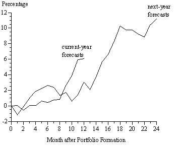
To explore the timing of these return differentials, Figure 1 shows the monthly cumulative difference between the performances of Portfolios 1 and 5, for portfolios based on current-year and next-year earnings predictions. The portfolios based on the current-year forecasts show little difference in cumulative returns through the eighth month after formation; the cumulative difference then spurts upward, from 0.9 percentage points at the end of December to 6.1 percentage points at the end of April, the period during which the fiscal-year earnings are reported. For portfolios based on next-year forecasts, the cumulative difference is only 2.0 percentage points 13 months after formation and then rises to 11.2 percentage points by the April 30 following the fiscal year for the earnings predictions. An 11.2 percentage-point difference over two years is roughly consistent with a 6.1 percentage-point difference over one year.

It is hard to imagine that this excess return is some kind of risk premium. Growth stocks not only have relatively uncertain cash flows but, because of their long durations, are also more sensitive to changes in required rates of return. Tables 3 and 4 show that the monthly returns for Portfolio 5 have a higher standard deviation than does Portfolio 1 and more systematic risk (as measured by beta in relation to the S&P 500).

The timing patterns documented in Figure 1 further indicate that the cumulative return differences between Portfolios 1 and 5 are not a risk premium. In particular, if it were a risk premium why would the return differential be concentrated in the second half of each holding period? A more plausible explanation is that stock prices adjust as investors learn that earnings will be closer to the mean than was predicted.

8. Summary

The empirical success of contrarian investment strategies may be due to insufficient awareness of regression to the mean—the tendency of extreme observations to exaggerate differences in the latent traits that generate the data. The logic of regression to the mean applies both to successive earnings and to the relationship between predicted and actual earnings. The latter is investigated here. We find persuasive evidence that relative earnings forecasts are systematically too extreme—too optimistic for companies predicted to do well and too pessimistic for those predicted to do poorly. The accuracy of these forecasts can be improved consistently and substantially by shrinking them toward the mean. We also find that, for both current-year and next-year forecasts, portfolios of stocks with relatively optimistic earnings predictions underperform portfolios of stocks with relatively pessimistic predictions. Most tellingly, the return differentials are concentrated in the second half of the holding period, when investors are learning that earnings will be closer to the mean than was predicted.

References

Basu, S., 1977, Investment performance of common stocks in relation to their price-earnings ratios: A test of the efficient market hypothesis, Journal of Finance, 32, 663–682.

Bauman, W. S. and R. Dowen, 1988, Growth projections and common stock returns, Financial Analysts Journal, 44, 9-80.

Chan, K., 1988, On the contrarian investment strategy, Journal of Business, 61, 147–163.

Chan, L., Hamao, Y. and J. Lakonishok, 1991, Fundamentals and stock returns in Japan, Journal of Finance, 46, 1739–1764.

DeBondt, W. F. M. and R. Thaler, 1985, Does the stock market overreact?, Journal of Finance, 40, 793–805.

DeBondt, W. F. M. and R. Thaler, 1987, Further evidence on investor overreaction and stock market seasonality, Journal of Finance, 42, 557–580.

DeChow, P. and R. Sloan, 1997, Returns to contrarian investment strategies: Tests of naive expectations hypotheses, Journal of Financial Economics, 43, 3–27.

Dreman, D. N. and M. A. Berry, 1995, Analysts forecasting errors and their implications for security analysis, Financial Analysts Journal, 51, 30–40.

Fama, E. F. and K. R. French, 1988, Permanent and temporary components of stock prices, Journal of Political Economy, 96, 246–273.

Fama, E. F. and K. R. French, 1992, The cross-section of expected stock returns, Journal of Finance, 47, 427–465.

Fama, E. F. and K. R. French, 2000, Forecasting profitability and earnings, Journal of Business, 73, 161–175.

Freeman, R. and S. Tse, 1992, “A Nonlinear Model of Security Price Responses to Unexpected Earnings.” Journal of Accounting Research 30(2): 185-209.

Hotelling, H., 1933, Review of The Triumph of Mediocrity in Business, Journal of the American Statistical Association, 28, 463–465; Secrist and Hotelling debated this further in the 1934 volume of this journal, 196–199.

Jaffe, J., D. Keim, and R. Westerfield, 1989, Earning yields, market values, and stock returns, Journal of Finance, 44, 135–148.

Kahneman, D., and A. Tversky, 1973, On the psychology of prediction, Psychological Review, 80, 237–251.

Keynes, J. M., 1936, The general theory of employment, interest and money (Macmillan, New York) 153–154.

King, W. I.,1934, Review of The Triumph of Mediocrity in Business by Secrist H., Journal of Political Economy, 42, 398–400.

Lakonishok, J., Shliefer, A. and R. W. Vishny, 1994, Contrarian investment, extrapolation, and risk, Journal of Finance, 49, 1541–1578.

La Porta, R., 1996, Expectations and the cross-section of stock returns, Journal of Finance, 49, 1715–1742.

Lintner, J., and R. Glauber, 1967, Higgledy, piggledy growth in America, presented to the Seminar on the Analysis of Security Prices, University of Chicago, May 1967, reprinted in: J. Lorie and R. Brealey, eds., 1978, Modern developments in investment management, 2nd ed. (Dryden, Hinsdale).

Little, I. M. D., 1966, Higgledy piggledy growth again (Basil Blackwell, Oxford).

Lord, F. M., and M. R. Novick, 1968, Statistical theory of mental test scores (Addison-Wesley, Reading).

Maddala, G. S., 1992, Introduction to econometrics, 2nd ed. (Macmillan, New York) 104–106.

McQueen, G., Shields K. and S. R. Thorley, 1997, Does the ‘Dow-10 investment strategy’ beat the Dow statistically and economically?, Financial Analysts Journal, 53, 66–72.

Nicholson, S. F., 1960, Price-earnings ratios, Financial Analysts Journal, 16, 43–45.

Nicholson, S. F., 1968, Price ratios, Financial Analysts Journal, 24, 105–109.

Poterba, J. M. and L. Summers, 1988, Mean reversion in stock returns: Evidence and implications, Journal of Financial Economics, 22, 27–59.

O’Higgins, M. B. and J. Downes, 1992, Beating the Dow (Harper Collins, New York).

Rosenberg, B., Reid, K. and R. Lanstein, 1985, Persuasive evidence of market inefficiency, Journal of Portfolio Management, 11, 9–17

Schmittlein, D. C., Surprising inferences from unsurprising observations: Do conditional expectations really regress to the mean?, The American Statistician, 43, 176–183.

Table 1 Current-Year Forecasts of Standardized Percentage Change in Earnings

Table 2 Next-Year Forecasts of Standardized Percentage Change in Earnings

Table 3 Five Portfolios Based on Current-Year Earnings Forecasts

Table 4 Five Portfolios Based on Next-Year Earnings Forecasts

Figure 1 Cumulative Difference Between Portfolio 1 and Portfolio 5 Returns after Formation